Overview

The goal of this challenge is to identify faults on seismic volumes and then build a polygon around them in three dimensions. We are providing the data for this challenge in a typical data science challenge format, but you aren't required to use machine learning to solve the problem.  

Background

Did you know that rocks can bend and break just like a toothpick? Due to the force of gravity, there is an immense amount of pressure in the earth's crust acting in all different directions. Over time this pressure will stress and deform the rocks. If the stress is high enough over a long enough time period the solid rock will deform in a ductile manner, bending and squashing like a piece of taffy on a hot summer day. However, if the stress is strong enough over a short enough time period, the rocks will break and deform in a brittle manner along what geoscientists call a fault. Once a rock breaks for the first time and creates a fault, subsequent movement of the rock due to the stress within the earth often continues to happen along these faults. The earthquakes we measure and feel today are evidence of this ongoing process of movement along these faults. 

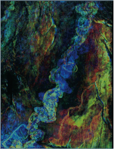
Figure 1. An RGB blend of a seismic volume from offshore West Africa. For this blend, the blue colors are high frequency, green colors are mid frequencies, and red colors are low frequencies. After Bahorich et al. (2002).

In the subsurface, faults can either be active and move, or they can be inactive and be records of past movement of the rocks. To image these faults we use seismic sound waves propagated into the earth and record their response as they reflect back to the surface as part of 2D and 3D seismic surveys. Faults appear different from the surrounding rocks. They usually are low amplitude, and generally offset the surrounding layers of rock. Some faults are very easy to identify, while others require additional seismic processing time to find and map. One useful process is called spectral decomposition (Figure 1). Think of spectral decomposition like a prism, where you shine white light on one side, and the light that comes out the other side is split into its respective wavelengths. For seismic data, spectral decomposition is usually performed on the frequency domain, and you can think of it as a measure of the seismic amplitude for a given frequency band. The results are traditionally visualized by blending any color you like to the different frequencies. 

For this challenge, we are asking you to find and map faults in 3D seismic volumes (Figure 2). You can choose to use spectral decomposition for additional features in your data engineering pipeline or not.

Figure 2. An example image of faults in a map-view time slice of a spectrally decomposed seismic volume.

Data and Labels

The data for this challenge are 400 3D seismic volumes and corresponding fault labels. The labels for each volume are structured as numpy array masks that identify every fault in every survey. Additionally we provide you with a test dataset you will use to make predictions which you will then submit for scoring.

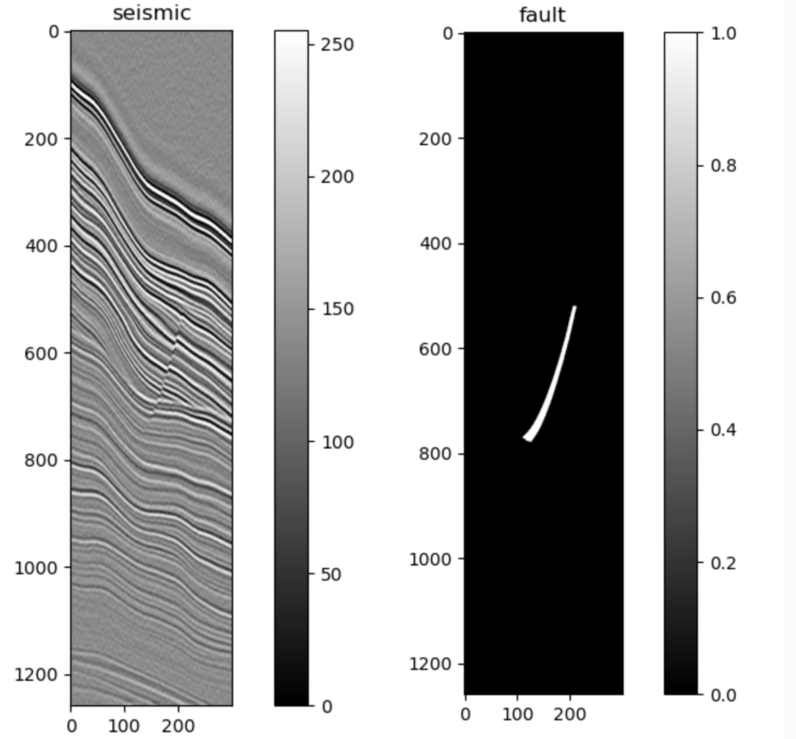
Figure 3. Cross section of a volume from the training dataset that documents the seismic amplitude and associated fault mask. Your job is to predict the mask on the right in three-dimensions.

Evaluation

For this challenge we will be using a Dice Coefficient (link) similar to the one we used for the Every Layer challenge (link). However, for this Challenge we will be using a 3D Dice Coefficient that takes your predicted fault masks and compares them to the ground truth fault masks.

Your submission will be an .npz file containing 50 arrays. This file format, used by NumPy, allows you to store multiple arrays in a compressed archive. Although it isn’t a dictionary, it functions similarly by storing key-value pairs, where each key is a sample ID from the test dataset and each value is an array representing the 3D coordinates of faults in that sample.

You will find a sample submission in the provided materials under the Data Tab. For more details on the submission format and naming conventions, please refer to the starter notebook. Additionally, the starter notebook includes a function to help you create the submission file from your fault predictions.

Final Evaluation

For the Final Evaluation, the top submissions on the Predictive Leaderboard will be invited to send Onward Challenges their fully reproducible Python code to be reviewed by a panel of judges. The judges will run a submitted algorithm on up to an AWS SageMaker g5.12xlarge instance, and inference must run within 4 hours. The Dice score metric used for the Predictive Leaderboard will be used to score final submissions on an unseen hold out dataset. The score on this hold out dataset will determine 90% of your final score. The remaining 10% of the final score will assess submissions on the interpretability of the submitted Jupyter Notebook. The interpretability criterion focuses on the degree of documentation (i.e., docstrings and markdown), clearly stating variables, and reasonably following standard Python style guidelines. For our recommendations on what we are looking for on interpretability see our example GitHub repository (link).

A successful final submission must contain the following:

• Jupyter Notebook: Your notebook will be written in Python and clearly outline the steps in your pipeline

• Requirements.txt file: This file will provide all required packages we need to run the training and inference for your submission

• Supplemental data or code: Include any additional data, scripts, or code that are necessary to accurately reproduce your results

• Model Checkpoints (If applicable): Include model checkpoints created during training so we can replicate your results

• Software License: An open-source license to accompany your code

Your submission must contain the libraries and their versions and the Python version (>=3.10).  See the Starter Notebook on the Data Tab for an example.

Timelines and Prizes

Challenge will open on 2 October 2024 and close at 23:00 UTC 8 January 2025. Winners will be announced on 21 February 2025. 

The main prize pool will have prizes awarded for the first ($10,000), second ($5,000), and third ($3,000) in the final evaluation. There will be two $1,000 honorable mentions for valid submissions that take novel approaches to solving the problem.

References

Bahorich, M., Motsch, A., Laughlin, K., & Partyka, G. (2002). Amplitude responses image reservoir. Hart’s E&P, January, 59-61.