Meta's Segment Anything Model (SAM) has many use cases that are being discovered even as you read this sentence. This model performs well at common segmentation tasks, but what are the next-generation use cases? For this challenge, you are tasked with one of these new use cases, using SAM to find all the layers, everywhere, all at once in 3D seismic data.

Background

Seismic data is a window into the Earth, and Geophysicists use seismic to identify and map different rock layers and structures.  A good analogy would be a radiologist using MRI data to diagnose a patient's ailment better.  There are numerous uses for seismic data, like reservoir identification and monitoring for CO2 sequestration, oil and gas exploration, and groundwater identification and management.  To make full use of seismic data, though, the different layers of the Earth need to be identified and mapped to be used as inputs to other analyses.  Creating maps of layers is the core of the challenge.  By speeding up this process, Geophysicists can interpret large amounts of data quickly and develop a better understanding of the Earth.

Standing in your way of this task is the seismic data itself.  Seismic can be challenging to understand because it is the complication of geology and the workflow used in collecting and processing the data.  Complex geology makes for more ambiguity in the seismic image and its interpretation.  For this challenge, the seismic data is relatively clean but still has many geologic features (faults, pinch outs, etc.) that an algorithm must learn how to interpret reasonably.

Challenge Structure

For this challenge, ~9,000 seismic volumes have been pre-interpreted with segment masks (labels) for your model to train on.  Each seismic volume has a unique assemblage of geologic features that your solution must consider.  The holdout data for this challenge will mirror the complexity of the Training data.

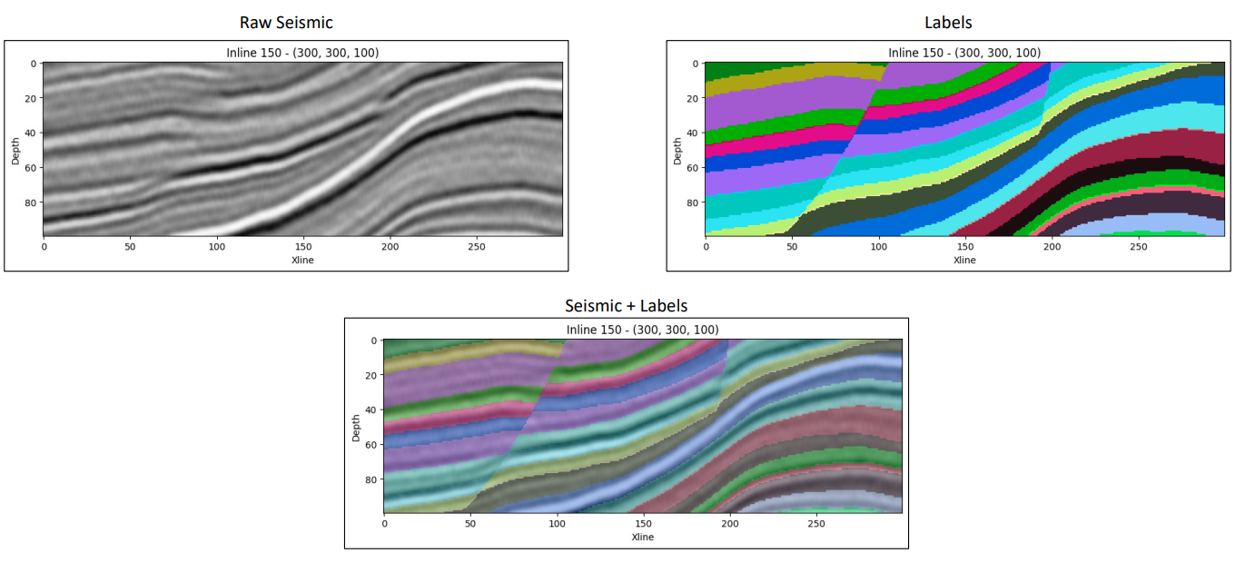
Figure 1: 2D slice of data (raw seismic), labels, and the two overlain.

Participants are free to build any pipeline for segmenting 3D data they feel comfortable with, but SAM must be involved in some part of the process.  For example, a solution could use UNET to generate the segments that feed into the SAM model for fine-tuning.  The output for a successful algorithm will be a NumPy array containing segment IDs for each labelled interval. Participants are free to slice, augment, or prepare the data however they deem fit.  This is a new space for these algorithms, so feel free to experiment.

Use as many training volumes as your solution needs.  The training volumes are divided into four tranches of files for more accessible download and experimentation.  We recommend starting with one tranche of data to get started.  We generated 9,000 training files to ensure abundant data for any solution a participant could want to build.

Evaluation

To evaluate the performance of your solution, you will need to submit segmentation masks for the 50 test volumes found on the Data Tab.  For this challenge, a Dice Coefficient is the primary metric to assess the accuracy of your model. You can learn more about Dice Coefficient scoring here (link).

 This challenge is unique because of the data's 3D nature, so the scoring algorithm has several evaluation steps:

1. A 2D slice is selected from a submitted volume; each segment in the slice is compared with its ground truth segment equivalent (see Table 1).

2. The false positives, true positives, and false negatives are calculated per segment for that slice.

3. Steps 1 and 2 are repeated for each slice in the submitted volume.

4. The false positives, true positives, and false negatives are summed for each segment in the volume, and then the Dice coefficient is calculated.

5. The Dice coefficient for each segment is averaged together, providing a final score for the volume.

6. Steps 1 through 5 are repeated for each of the 50 test volumes.  The average Dice coefficient of all 50 test volumes is then calculated for the Predictive Leaderboard score.

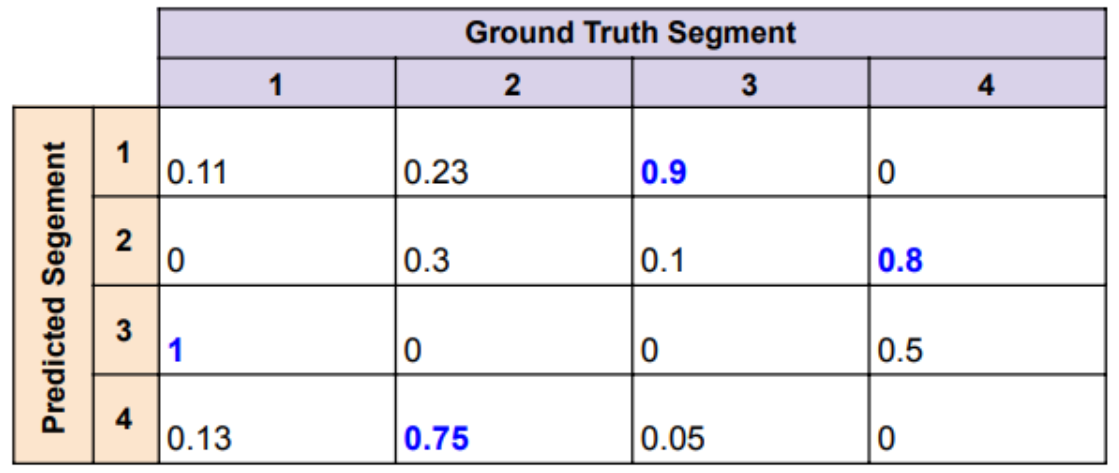
Table 1: Example of the matching between predicted and ground truth segments.

Please note that the submission file naming convention must be used for the scoring algorithm to work correctly. For example, predictions for 'test_vol_1.npy', 'test_vol_2.npy'... 'test_vol_50.npy' must be named as 'sub_vol_1.npy', 'sub_vol_2.npy'... 'sub_vol_50.npy' files, respectively. The Data Tab has a sample submission file for the Test Data set.  

Final Evaluation

For the Final Evaluation, the top submissions on the Predictive Leaderboard will be invited to send Xeek their fully reproducible code to be reviewed by a panel of judges. The judges will run the submitted algorithm on a series of holdout data and use the Dice coefficient method to determine the best-performing model. This score will be used for 95% of the user's final score. The remaining 5% of the final score will assess submissions on the interpretability of their submitted Jupyter Notebook. The interpretability criterion focuses on the degree of documentation (i.e., docstrings and markdown), clearly stating variables, and reasonably following standard Python style guidelines.  

A successful final submission must contain the following:

• Jupyter Notebook with a clearly written pipeline.

• Requirements.txt file that instructions on how to run training/inference for the submission

• Any supplemental data or code to reproduce your results.  

 It must contain the libraries and their versions and the Python version (>=3.6). 

See the Starter Notebook on the Data Tab for an example.

Prizes

The main prize pool will have prizes awarded for the first ($24,000), second ($15,500), and third ($9,500) in the final evaluation. Two $1,000 honorable mentions will also be awarded for submissions that show novel data pre-processing workflows, implementations of SAM, or processing pipelines.