Overview

Scale is one of the more interesting aspects of science.  Biology investigates genomes and entire ecosystems.  Physics spans quantum forces to gravitational waves from the Big Bang.  Understanding all the different scales for a problem helps us better understand our natural world and how it is changing.  For this challenge, we're asking you to investigate the micrometer scale of geosciences by examining thin sections of rocks and identifying their components.

This challenge aims to build a machine-learning solution to interpret different kerogen macerals.  This challenge is the sequel to the Stranger Sections Challenge, exploring unsupervised segmentation of thin section images. In Stranger Sections 2, challengers will receive labeled training data and a larger test set of images.  You will have to devise different methodologies to find the right labels. This challenge has five honorable mention prizes to reward participants' efforts in finding new paths to solve this problem.

Background

Biological uses for microscopes are widely understood: understand human cells or a parasite in a water sample.  Geoscientists also use microscopes in their day-to-day work to identify mineral types in aquifer rock samples or the structure of crystals in granite.  In this challenge, you will be tasked with building a model that correctly segments and classifies a particular maceral type, kerogen, in reflected light polished sections.

Reflected light microscopy is the study of minerals with light projected down onto the polished section. It is slightly different than a traditional microscopy and occurs when minerals are opaque, like kerogen macerals. Kerogen is an insoluble organic matter in sedimentary rocks [1].  Kerogen forms when plants, algae, or other microorganisms die and are buried in sediment.  Geologic processes like heat and pressure transform the organic material into kerogen.  Several types of kerogen exist, each containing different types of organic material.  The organic material and chemical makeup of kerogen help scientists understand the paleo-environments and a hydrocarbon deposits' type, quality, and chemical composition.  This can all be important information for teams of scientists and engineers looking for new hydrocarbon reserves [2].

Kerogen can be divided into 3 groups: liptinite, vitrinite, and inertinite. Each of these groups were deposited in different paleo-environments and also have different characteristics under a microscope. Liptinite, also known as Exinite, can contain Type I and II kerogen with sources from marine, lacustrine, and terrestrial environments. Vitrinite is a Type III kerogen and comes from terrestrial environments, composed of mostly woody materials. Finally, Inertinite is a Type III coaly kerogen composed of recycled materials plus plant materials that have undergone natural carbonization such as charring, oxidation, moldering, and fungal attack [3].

Below is a table highlighting important characteristics of the three types of kerogen macerals: liptinite, vitrinite, and inertinite. Included in this table are descriptions of what these samples will look like under plain and UV lights.

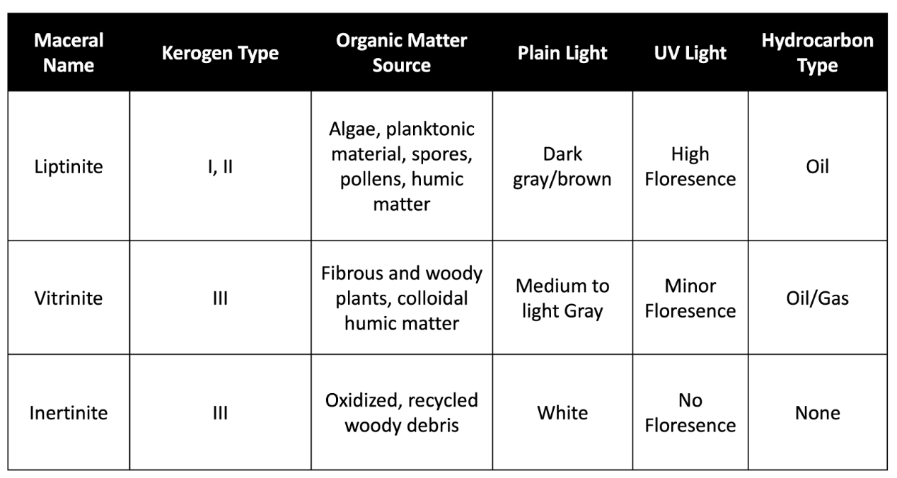
Figure 1. Table describing kerogen maceral characteristics

Data

This challenge has three kerogen types: Liptinite , Virinite, Inertinite.  See Figures 1-3 below for examples of each maceral type. The data for this challenge consists of a training dataset, a test dataset, and additional unlabeled data. The training dataset consists of 87 images with segmentation mask labels. These images from the training dataset will be split into 3 classes; 42 Liptinite, 27 Vitrinite, 22 Inertinite. Please note that some images may contain multiple classes. The test dataset consists of 25 images without segmentation mask labels. The additional unlabeled data consists of 8641 images without segmentation mask labels. The additional unlabeled images contain all three classes for prediction, as well as other objects, like pyrite minerals. The images are provided as .jpg files of size (1024,1360) with 3 channels, and the size of the images are 172x228 microns. Macerals less than 10 microns in size do not need to be segmented. Training data labels are provided as Numpy arrays. Participants are free to augment or preprocess the data as they see fit.

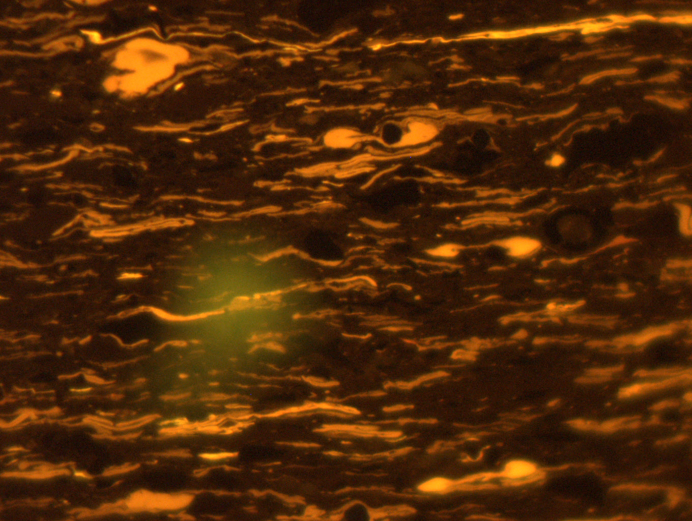
Figure 1. Liptinite macerals in UV Light

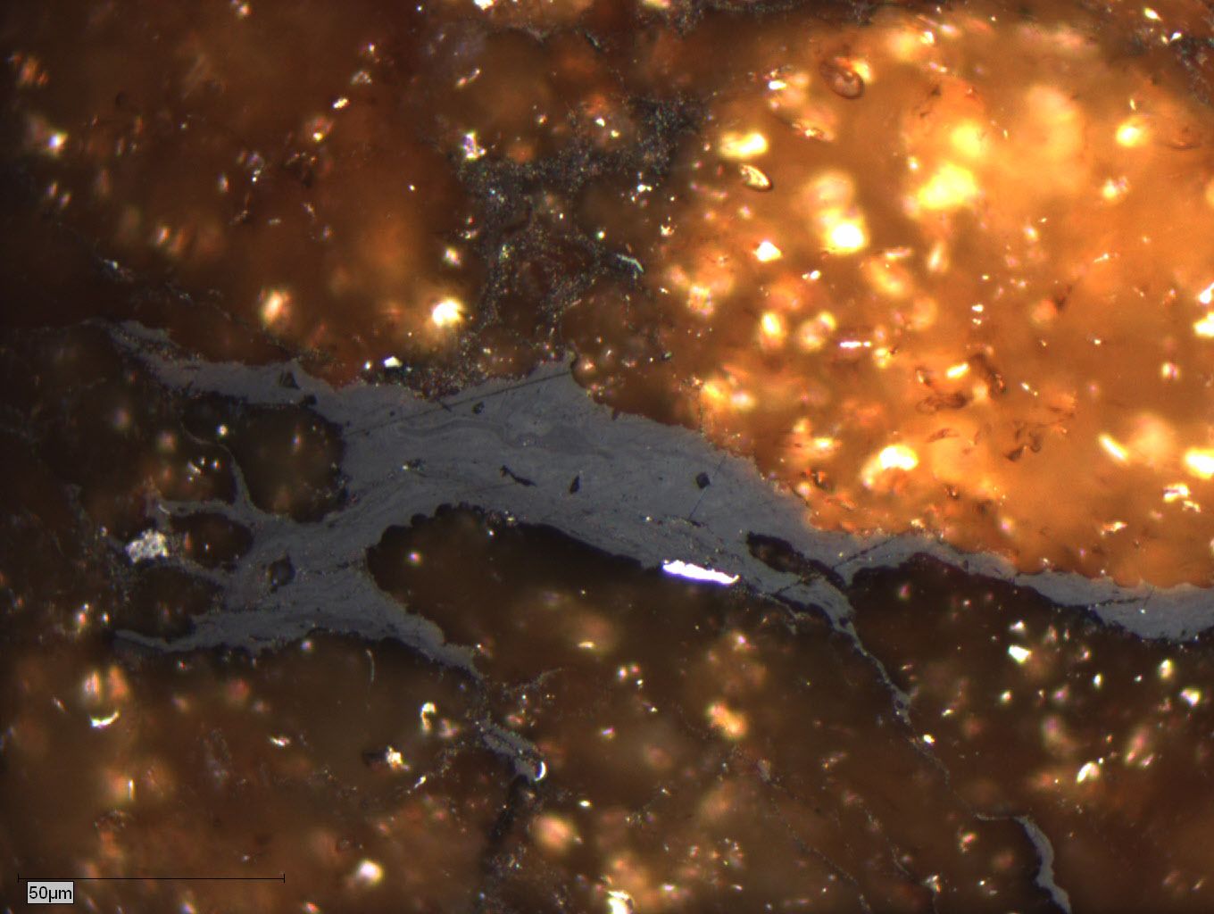
Figure 2. Vitrinite macerals in plain light 

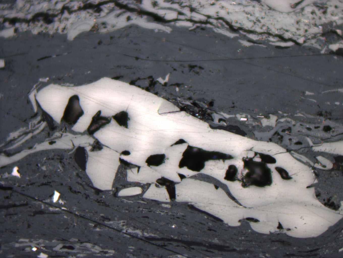
Figure 3. Inertinite maceral in vitrinite matrix in plain light

There are a small number of labels for these classes, therefore, you'll need to use different data science techniques to find ways to accomplish the goals of the challenge.  Transfer learning, data augmentation, and unsupervised learning are all techniques that can be employed.

Evaluation

To evaluate the performance of your solution you will need to submit segmentation masks for the 25 test images found on the Data Tab. For this challenge, a Dice Coefficient or Jaccard Score is the primary metric to assess the accuracy of your model. The live scoring algorithm uses the Scikit-learn implementation of jaccard_score() with average="micro" and can be read about here.

Please note that the submission file naming convention must be used for the scoring algorithm to work correctly. Each image has a unique 6 character id for it's name. It is important that when you create predictions for the images, the predictions are labeled in this format: `<image_id>_pred.npy`. For example, predictions for `1knjzt.JPG, 20di1f.JPG...ont2xr.JPG` must be named as `1knjzt_pred.npy, 20di1f_pred.npy...ont2xr_pred.npy` files, respectively. The Data Tab has a sample submission file for the Test Data set. The example submission file provided on the Data Tab is to purely for your reference, not to be used in your prediction pipeline. Each submission file must contain a segmentation mask for whole image - make sure that dimensions of your prediction match the shape of test volume.

Final Evaluation

At the end of the challenge, Onward will request the models from the top submissions on the Predictive Leaderboard for review by a panel of judges.  For the main prize pool, the Judges will run the submitted algorithm on a series of holdout data to determine the best-performing model.  The score on the hold out data will be used for 95% of the user's final score. The remaining 5% of the final score will assess submissions on the interpretability of their submitted Jupyter Notebook.  The interpretability criterion focuses on the degree of documentation (i.e., docstrings and markdown), clearly stating variables, and reasonably following standard Python style guidelines (PEP8). 

Final submissions must contain:

• Jupyter Notebook: your notebook should clearly outline the steps in your pipeline

• Requirements.txt file: This file should provide instructions on how to run the training and inference for your submission, and must contain the libraries and their versions and the Python version (>=3.9).

• Supplemental data or code: Include any additional data, scripts, or code that are necessary to accurately reproduce your results

• Model checkpoints: A model checkpoint file from the end of your model training process

The judges will run the submitted algorithm on AWS SageMaker, and will use up to a g5.24xlarge instance. Model inference must run within 24 hours. If the code cannot run in the allotted time, the challenger will be notified and given 24 hours to make edits. If no edits are made, the submission will be disqualified.

Timeline and Prizes

The challenge will open on March 25 2024 and close at 22:00 UTC June 28 2024.

The main prize pool will have prizes awarded for the first ($10,000), second ($6,000), and third ($4,000) in the final evaluation.  Five $2,000 honorable mentions will also be awarded for different categories (see Final Evaluation).  A participant can be awarded prizes from the main prize pool and multiple honorable mentions depending on the quality of their submission. 

References

[1] https://en.wikipedia.org/wiki/Kerogen

[2] https://wiki.aapg.org/Kerogen

[3] Hunt, J.M. (1979) Petroleum Geochemistry and Geology. W.H. Freeman and Company, San Francisco, p. 274-276