Overview

Welcome to an exciting trip into the world of oil and gas production. Our journey takes us deep beneath the earth's surface, where we collect bottom hole pressure data. The dataset for this challenge is a wealth of information, poised to reveal insights into the dynamics of energy production.

Just like the Ghosts of Holiday Past challenge, this challenge is focused on time series data. These bottom hole pressure data are one of the keys to understanding the intricacies of energy production. These data hold information about patterns, anomalies, and potential opportunities. By deciphering the intricacies of bottom hole pressure, you will gain valuable insights that allow optimization, improved safety, and increased efficiencies. 

For this challenge we have provided you with a set of 1D bottom hole pressure time series data for oil and gas production and water injection. Your task is to predict if a well is flowing or not, given the bottom hole pressure. 

Background

The data for this challenge are bottom hole pressure time series from oil and gas wells. Bottom hole pressures are key metrics in energy production, as they document the pressures present deep within the earth's subsurface reservoirs. These pressures in turn help characterize the interactions between rock formations and the fluids moving within them. By monitoring and analyzing bottom hole pressures, we can optimize well design, production rates, and maximize the fluid recovery from each well. Understanding and monitoring these pressures also helps us detect for wellbore instability or formation damage. This helps us safeguard personnel, protect the environment, and mitigate potential hazards. 

The data contains measurements of the pressure at the bottom of each well in one minute intervals. These data show how the pressure in each well changes when they are opened and closed (flowing and shut in, respectively) over time (Figure 1). For producing wells, pressures generally rise while shut in, and decrease while flowing. For injection wells, the opposite is true, pressures generally rise while injecting, and decrease while shut in.  Due to sensor issues some of the data in the time series are erroneous or missing. 

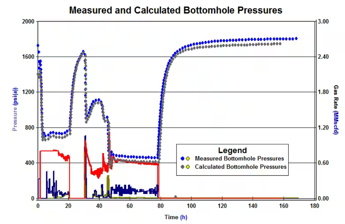
Figure 1: Pressure plot showing different patterns in pressure as a well is shut in.  From Milovanov (2017).

This challenge asks you to build a model to predict if a well is flowing or shut in. The model should take into account the shape of the time series, and the pressure values over time. Keep in mind that we consider producing and injecting wells, so increases or decreases must be identified depending on the case. 

Data

The dataset provided for this challenge consists of time-series bottom hole pressures from 200 oil and gas wells. They can correspond to producing or injecting wells, so shut ins correspond to increases or decreases depending on the case. Each well has a unique profile that represents the geology, completions, and operations of the well. Figure 2 shows two of these wells with the associated flowing and shut in labels.  Use these labels to build your predictive model.  However, be cautious of overfitting as the holdout data for this challenge will be more diverse than what is in the train and test set. One of the goals of this challenge is to create a generalizable model that can be deployed in many different data conditions.

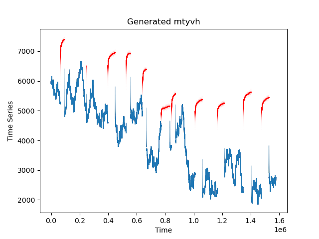
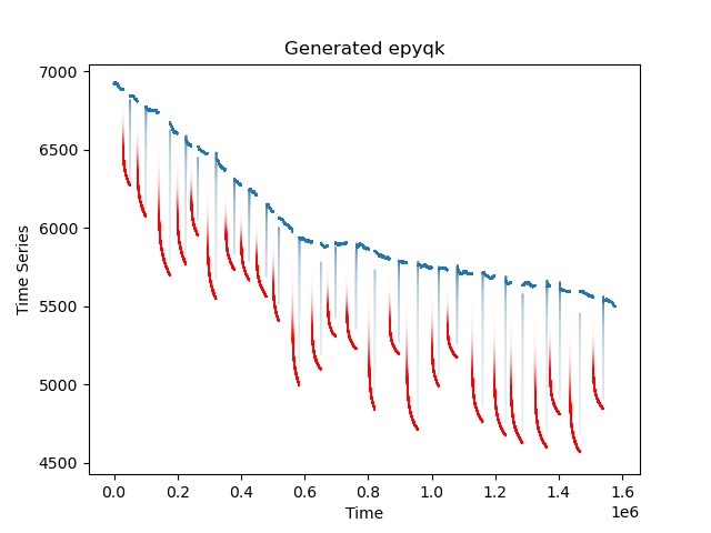
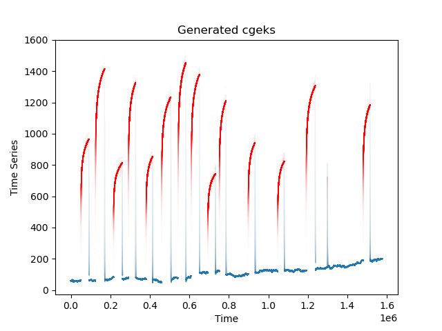
Figure 2. Example of bottom hole pressure plots with labels.

Evaluation

To evaluate your solution's performance, you'll need to submit a JSON file containing the predicted intervals for the holdout dataset. This submission should be structured as follows {file_name_1 : [l1, l2, …], file_name_2 : [l1, l2, …]} in which each file_name corresponds to the well name and each predicted_interval li is a tuple in the form (start_i, stop_i). Evaluation of your submission will use a weighted score:

Where

are weights of 1, 3, and 2 respectively. 

IoU is an averaged intersection over union (link) which compares the total intersections of the predicted intervals (li) to the total unions (Lj) across all paired intervals.

Next, Fβ is defined as:

Where β=0.5 to give more importance to Precision than Recall, Recall is the recall rate, which in this case is the number of predicted shut-ins that match actual shut-ins divided by the number of actual shut-ins. Precision is the precision, which is the number of predicted shut-ins that match actual shut-ins divided by the number of predictions. 

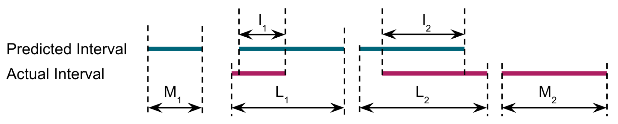
Thus, for the example in Figure 3, Recall = cardinality ({l1, l2}) / cardinality ({L1, L2, M2}) = 2/3 and 

Precision =  cardinality ({l1, l2}) / cardinality ({M1, l1, l2}) = 2/3

Start_error is an exponential decay of the time between the predicted shut-in start and the actual shut-in start:

Where true_start is the actual shut-in start time, predicted_start is the predicted shut-in start time, n is the number of shut-ins, and tau=5 if predicted_start > true_start and tau=10 otherwise.

We've included a sample_submission_generator() function in the utils.py module that generates and saves a sample submission file in JSON format (with random classifications), illustrating the expected format. Additionally, you'll find a sample submission file in the sample_submissions folder. 

To aid your understanding, we've provided code examples of every process and analysis step, as well as the scoring algorithm, in the starter notebook, demonstrating how submissions are evaluated and scores are calculated. Submissions are limited to a maximum run time of 15 minutes to score.

Final Evaluation

At the end of the challenge, Onward will request the models from the top submissions on the Predictive Leaderboard for review by a panel of judges.  For the main prize pool, the Judges will run the submitted algorithm on a series of holdout data to determine the best-performing model.  The score on the hold out data will be used for 95% of the user's final score. The remaining 5% of the final score will assess submissions on the interpretability of their submitted Jupyter Notebook.  The interpretability criterion focuses on the degree of documentation (i.e., docstrings and markdown), clearly stating variables, and reasonably following standard Python style guidelines (PEP8). 

Final submissions must contain:

• Jupyter Notebook: your notebook should clearly outline the steps in your pipeline

• Requirements.txt file: This file should include all the packages and modules to run the training and inference for your submission. We recommend the pipreqs package to generate this file. Python version should be >=3.9.

• Supplemental data or code: Include any additional data, scripts, or code that are necessary to accurately reproduce your results

• Model checkpoints: A model checkpoint file from the end of your model training process

The judges will run the submitted algorithm on AWS SageMaker, and will use up to a g5.12xlarge instance. Model inference must run within 24 hours. If the code cannot run in the allotted time, the challenger will be notified and given 24 hours to make edits. If no edits are made, the submission will be disqualified. 

Timelines and Prizes

Challenge will open on March 25 2024 and close at 22:00 UTC June 28 2024.

There will be a total prize pool of $30,000 for this challenge.  There will be different prize levels for challenges:

• First place ($15,000)

• Second place ($8,500)

• Third place ($5,500)

• Two honorable mentions ($500)

References

Milovanov, V. (2017, August 10). Using surface recorders to monitor the progress of transient pressure tests.  S&P Commodity Insights. https://www.spglobal.com/commodityinsights/en/ci/research-analysis/using-surface-recorders-to-monitor-the-progress-of-transient-pressure-tests.html