
Artificial Intelligence
Generative AI
Unsupervised Learning
Completed
No Second Guessing
$15,000
Completed 2 weeks ago
164 teams
Overview
Let’s be real: nobody wants to spend fourteen days with their agents grinding on a dataset just to get played by a honeypot. In this challenge, we’ve rigged the dataset with digital potholes. These are fake pay zones that look like real but are actually just rock bottom. If your agent isn't cut for it, it’s going to take an L. We’re putting up a payout for the person who can build an agent so confident it can do a hundred meter dash through these curves with its hands in its pockets. No luck required, this challenge is all about rock solid logic, so you never have to second guess if you’re hitting pay or just hitting a wall.
Agentic workflow detecting all pay zones, ignoring decoys
Your goal is to develop an agentic workflow that identifies every single pay zone in the vertical well log curves with one hundred percent accuracy. The challenge closes when a single team scores 100 on the predictive leaderboard or after 14 days, whichever comes first. Filter out the noise and decoys so every submission moves you closer to the win. Miss one calculation, and the dream of perfection ends. Build your system to finish clean.
⚠️ This is not a traditional Challenge.
There is no starter notebook, no benchmark model, and no pre-processed training data. That's by design. This challenge asks you to build an agentic workflow from scratch. Your system should ingest raw, unconditioned LAS files and produce a complete petrophysical suite without hand-holding. What you do get:
Raw LAS files: A stack of wells in their original, unprocessed state
Submission Curves: You will submit the following curves for scoring on each well,
VSH,PHIT,PHIE,SW,PERM, andPAY_FLAG
That's it. The rest is up to you and your agent. Interested? Read on for details.
Background
This challenge involves vertical well log curves which are data points governed by the principles of petrophysics and fluid dynamics. If you don’t know a gamma ray from an X‑ray, think of a well log as the raw telemetry from a network: it’s a stream of signals you interpret to tell what’s really happening underground. The curves (Figure 1.) are the data points telling us if the rock is porous (space for the good stuff) or permeable (lets the good stuff move). A pay zone is the ultimate vibe check where the rock is actually holding value. The catch? The subsurface is full of fakes. These are layers that look like pay but are actually just tight, useless rock.
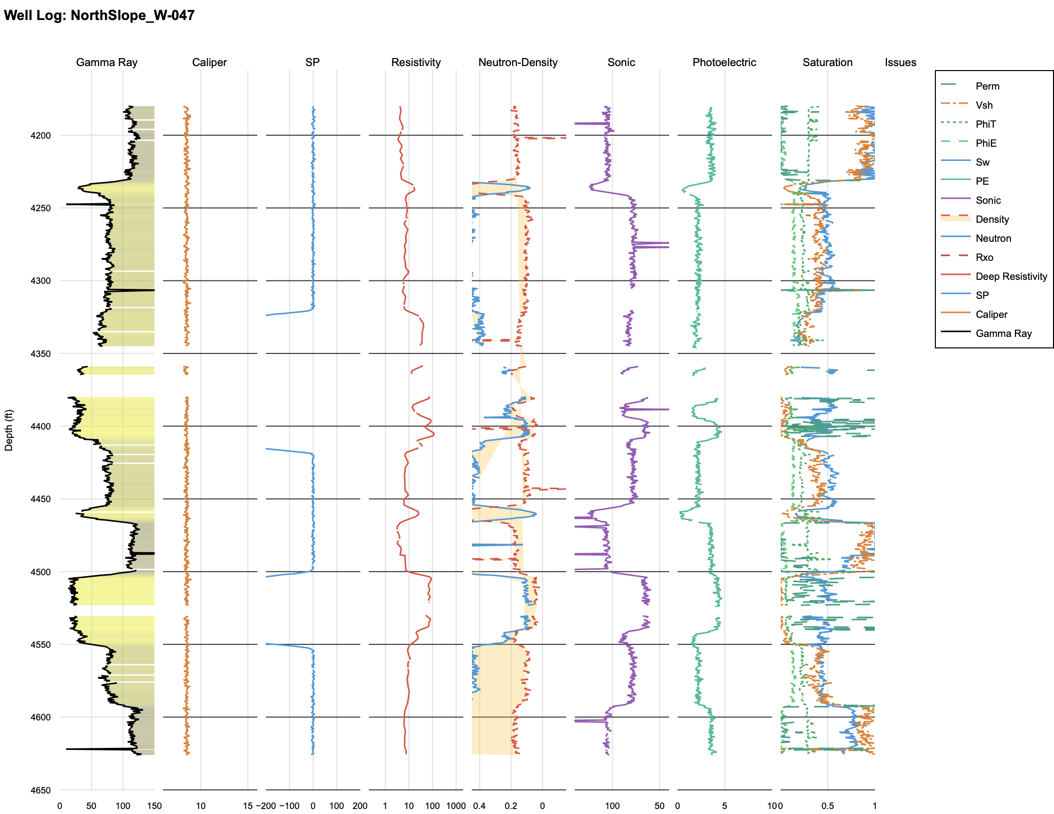
Figure 1. Example of well-log curves after being processed through a standard petrophysical workflow. These are the curves you will need to include in your submissions.
Identifying these zones is a classic inverse problem where you are given the resulting measurements and must work backward to reconstruct the physical reality of the subsurface. Geological formations are inherently noisy and data can be ambiguous. Traditional approaches often fall short because a single misinterpretation can lead to a dry hole.
Success in this challenge requires moving beyond simple thresholding and hand built models. The most effective solutions will utilize agentic workflows to peer through the noise. Your system needs to act like a seasoned petrophysicist by filtering out decoys and identifying the pay with surgical accuracy. You are building a system designed to finish clean every single time. Check out this repo for some ideas and skills that might come in handy later.
Data
The dataset consists of raw well log files provided in LAS format with no pay flag or lithology labels. These logs represent various vintages and include a diverse range of curves that reflect different acquisition standards and historical recording methods. This variety requires a robust ingestion pipeline capable of handling inconsistent headers and mnemonic variations.
Your task is to build a full end-to-end pipeline that processes these raw LAS files and generates a complete petrophysical log suite. The final output must also be submitted as LAS files. This suite must include lithology classifications, pay flags, and all intermediate curves used to derive those flags.
A submission sample is provided to help your agent get the formatting correct. Every well should have VSH, PHIT, PHIE, SW, PERM, and PAY_FLAG curves. Your system must demonstrate the ability to transform raw, unconditioned data into a standardized and actionable petrophysical product.
Some info on the data:
800 wells total: 75% real, 25% honeypots. You do not know which is which.
5 submissions per day for 14 days = 70 maximum submissions.
Each submission must contain processed LAS files for all wells.
Evaluation
Your final score is the geometric mean of four equally weighted axes, each scored 0 to 100:
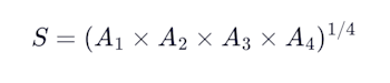
Neglecting any single axis is a bad idea. The geometric mean ensures a zero on one axis zeros your entire score.
The following notation is used throughout:
Symbol | Definition |
N | Total number of wells |
Nᵣ | Number of real wells |
Nₕ | Number of honeypot wells |
G | Number of physics gates per well |
gᵢ | Number of gates passed by well i |
Fᵢᵖʳᵉᵈ | Predicted net pay footage for well i (total feet where PAY_FLAG = 1) |
Fᵢᵗʳᵘᵉ | Answer key net pay footage for well i |
Pᵢᵖʳᵉᵈ | Set of depth samples where the submission flags pay for well i |
Pᵢᵗʳᵘᵉ | Set of depth samples where the answer key flags pay for well i |
τ꜀ | Scoring tolerance for curve c |
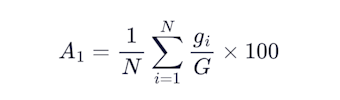
Axis 1: Gate Compliance
Every well is evaluated against G = 25 physics-based logic gates. These gates encode hard physical constraints that any valid petrophysical interpretation must satisfy (e.g., porosity cannot exceed 1.0, water saturation must be bounded between 0 and 1, permeability must be non-negative). Each gate returns a binary pass/fail for every depth sample in the well. A well's gate score is the fraction of gates passed, and your axis score is the average across all N wells:
Skipping a gate by not computing a curve won't help. If a computed curve exists in your submission but is 100% NaN, that's a failed gate. And if your submission has zero valid computed curves for a well, that well's gate score is zero, period. Submitting only GR + DEPTH + PAY_FLAG is not a petrophysical submission. You'll pay for missing curves on the other axes too. There is no free lunch.
Axis 2: Pay Accuracy
On the Nᵣ real wells, your net pay footage Fᵢᵖʳᵉᵈ is compared to the answer key Fᵢᵗʳᵘᵉ. The answer key uses standard petrophysical cutoffs for pay in a clastic reservoir. PAY_FLAG must be 0 or 1. Non-binary values will be rounded to the nearest integer before scoring.
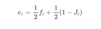
Each well i is scored by two components, equally weighted:
Footage error (50%): How close is your total net pay footage to the answer key?
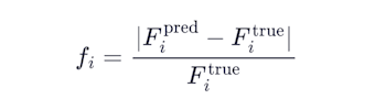
Jaccard overlap (50%): How well do your flagged pay depths overlap with the answer key's pay depths? If you get the total footage right but flag it in completely wrong depths, you only get half credit on that well.
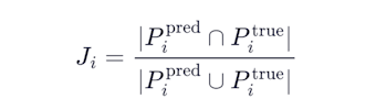
The combined per-well error is:
and the axis score is:
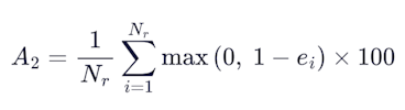
Overpredicting pay is penalized just as heavily as underpredicting it. If your submission doesn't cover the full depth range, a coverage penalty kicks in. Deleting data is not a path to a good score.
Axis 3: Honeypot Rejection
Certain wells contain physics violations baked into the raw measurements. A correct workflow produces zero pay on these wells. Each honeypot well i is scored as a binary. Any non-zero pay is a failure:
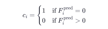
The axis score applies a power penalty to the fraction caught:
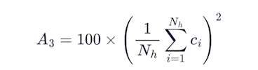
Notice the square in there. No linear averages here. Missing 3 of 30 honeypots doesn't cost you 10 points, it costs you 19. Missing 10 drops you to 44.4. The penalty bites harder the more you miss.
You don't know which wells are honeypots; your workflow must catch them from the physics. And if you try to game this by flagging zero pay on every well, A₂ = 0 and your final score is zero. The geometric mean makes that strategy a bad time.
Axis 4: Petrophysical Accuracy
On the Nᵣ real wells, three computed curves are compared to the answer key at every depth sample within Pᵢᵗʳᵘᵉ. The following table maps each LAS mnemonic to its mathematical symbol and scoring tolerance:
LAS Mnemonic | Symbol | Curve c | Tolerance τ꜀ | What it means |
PHIE | ϕₑ (effective porosity) | 1 | 0.03 v/v | 3 porosity units |
SW | S_w (water saturation) | 2 | 0.10 v/v | 10 saturation units |
PERM | log₁₀ k (log-permeability) | 3 | 0.50 log-decades | Your perm can be off by ~3x |
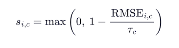
For each real well i and each curve c, the RMSE between your submitted values and the answer key is computed over all depth samples in Pᵢᵗʳᵘᵉ. The per-well, per-curve score is:
The per-well score is the geometric mean of the three curve scores:
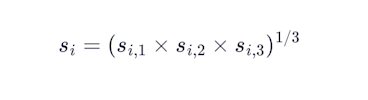
and the axis score is:

The geometric mean here is deliberate and mirrors the final score formula. A zero on any curve zeros the entire well. Porosity, saturation, and permeability are not independent outputs. They are linked by the same rock physics. A submission that nails porosity but cannot estimate permeability has not demonstrated petrophysical competence on that well.
These are generous tolerances. They correspond to competent petrophysicist accuracy, not an exact match. But you must actually submit data for the full well. If less than 50% of the pay interval is covered, that well is hard-zeroed. If more than 50% of a curve's values are NaN in the pay zone, that curve is hard-zeroed. Physically impossible values (negative porosity, SW > 1) get penalized multiplicatively. 50% out-of-bounds samples zeroes the curve entirely. Missing samples are treated as maximum error. You are heavily penalized for gaps in your output.
Final Evaluation
The evaluation dataset for this challenge contains both public and private (holdout) samples combined into a single dataset. You are required to generate and submit predictions for all samples with each submission. The assignment of samples to the public and private subsets is not disclosed.
During the competition, the Public Leaderboard reflects your performance on a subset of the evaluation data (the public subset). This leaderboard is updated based on your submissions and provides feedback on your model’s performance. Please note that the public leaderboard is computed on only a portion of the evaluation data and does not reflect your final ranking.
At the close of the competition, the Private Leaderboard will be revealed. Final rankings are determined based on your performance on the private (holdout) subset, using your highest-scoring submission on the Public Leaderboard.
Your private (holdout) score is not visible during the competition, and may differ from your public leaderboard score. It is common for rankings to change between the public and private leaderboards, as the final evaluation is performed on a different subset of the data.
Please note the following:
Final rankings are determined solely by holdout performance, not by the public leaderboard score.
The public leaderboard should be interpreted as directional feedback only, and may not perfectly reflect final standings.
Assuming reasonable representativeness between the public and holdout subsets, performance on the holdout set is expected to correlate with public leaderboard performance for models that generalize well.
Any attempt to infer or reverse-engineer whether specific samples belong to the public or holdout subsets is strictly prohibited and may result in disqualification. Participants are expected to focus on building models that generalize across the dataset as a whole.
Top-ranked participants on the private leaderboard will be invited to submit fully reproducible Python code for their solutions, which will be reviewed by a panel of judges.
The score achieved on the private leaderboard will determine 80% of the user's final score. 10% of the users score will be based on the participants approach to solving the problem. The remaining 10% of the final score is based on the interpretability of the user’s submitted code and skills.
A successful final submission should contain the following:
Python code: Your pipeline will be written in Python with clearly outlined steps.
README: A README file documenting your approach, architecture decisions, and instructions for reproducing your results end to end.
Requirements.txt file: This file will provide all required packages needed to run the training and inference for your submission. We recommend uv for package management.
Supplemental data or code: Include any additional data, scripts, or code that are necessary to accurately reproduce your results.
Agent documentation and configuration: Include your agent SKILL.md files and any additional artifacts required to reproduce your agentic workflow.
Model and harness disclosure: Specify the exact model(s) used and the harness/framework used to run the agents.
Model Checkpoints (If applicable): Include model checkpoints created during training so we can run your model
Software License: An open-source license to accompany your submission
Your submission must contain the libraries and their versions and the Python version (>=3.11).
Timelines and Prizes
Challenge will open on 17 June 2026 and close at 22:00 UTC 1 July 2026 or when the first participant reaches a score of 100 on the predictive leaderboard, whichever happens first. Winners will be announced on 15 July 2026. The main prize pool will have prizes awarded for first ($15,000) in the final evaluation.